The Tax Trap: Why the 2026 Budget May Actually Hurt New Build Investors

The 2026 Federal Budget changed the taxation of established properties. New builds purchased after 7:30 pm AEST on 12 May 2026 retain annual negative gearing and the 50% CGT discount. Established properties purchased after that date will lose both from 1 July 2027.

On the surface, that appears to settle the new-build vs established question. The reality is more nuanced. 

Tax treatment is one factor in investment performance, not the whole picture. It shapes how much of an investor’s return is retained after tax, but it does not determine the size of the underlying gain. 

A larger gross gain, taxed less favourably, could still outperform a smaller one taxed more favourably. In addition, the size of the gross gain depends primarily on market fundamentals that tax incentives cannot influence.

This blog tests the post-budget case for new builds across 3 sections. It begins with our theory of what could unfold across new-build markets, then models the dollar impact of that theory over a 10-year hold, and closes with a historical case study showing a similar dynamic across Australian markets.

Section 1: Our Theory on what could unfold

This section walks through the chain of events we think could unfold across many new-build markets post-budget. 

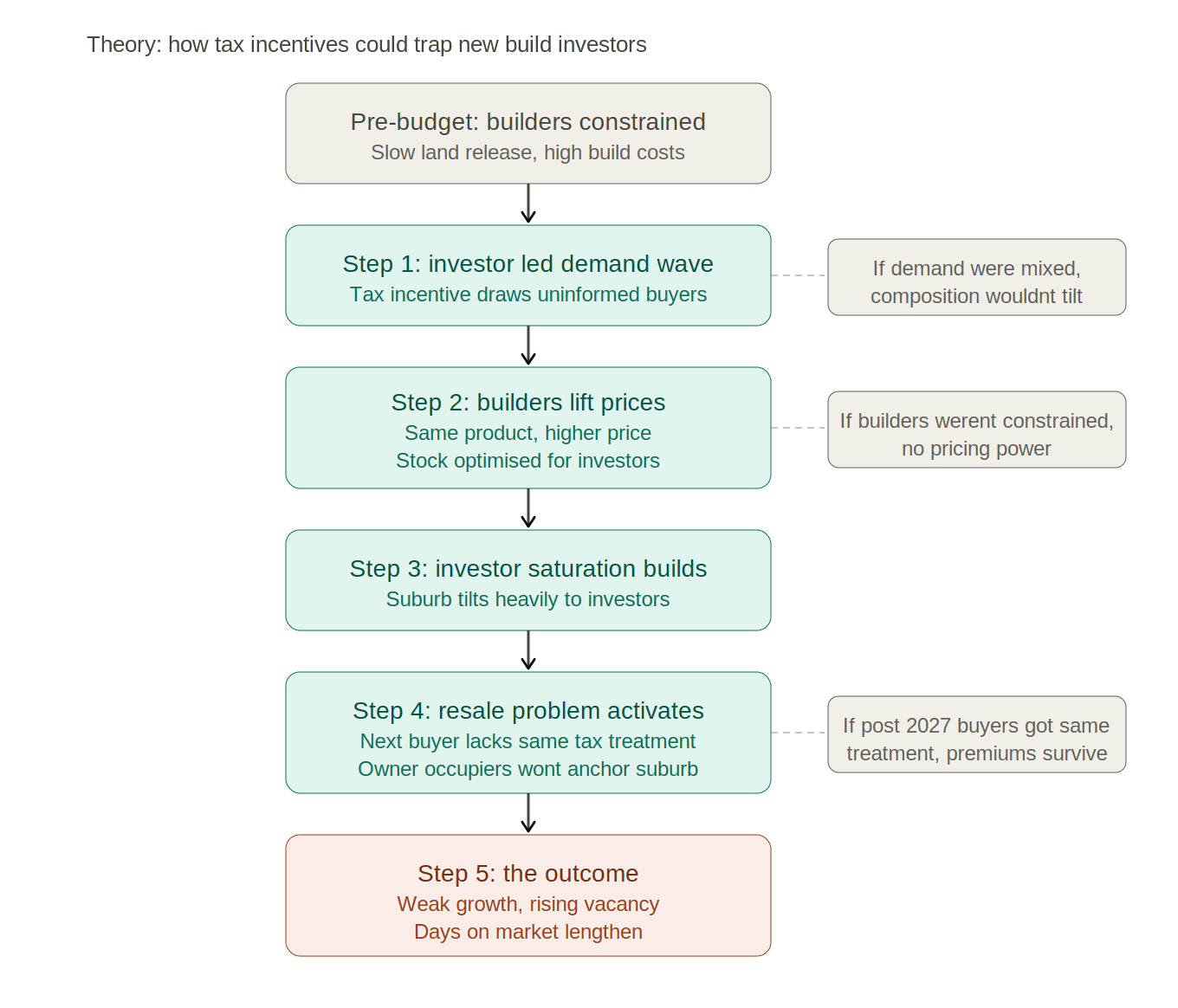
Pre-budget, builders were already constrained.

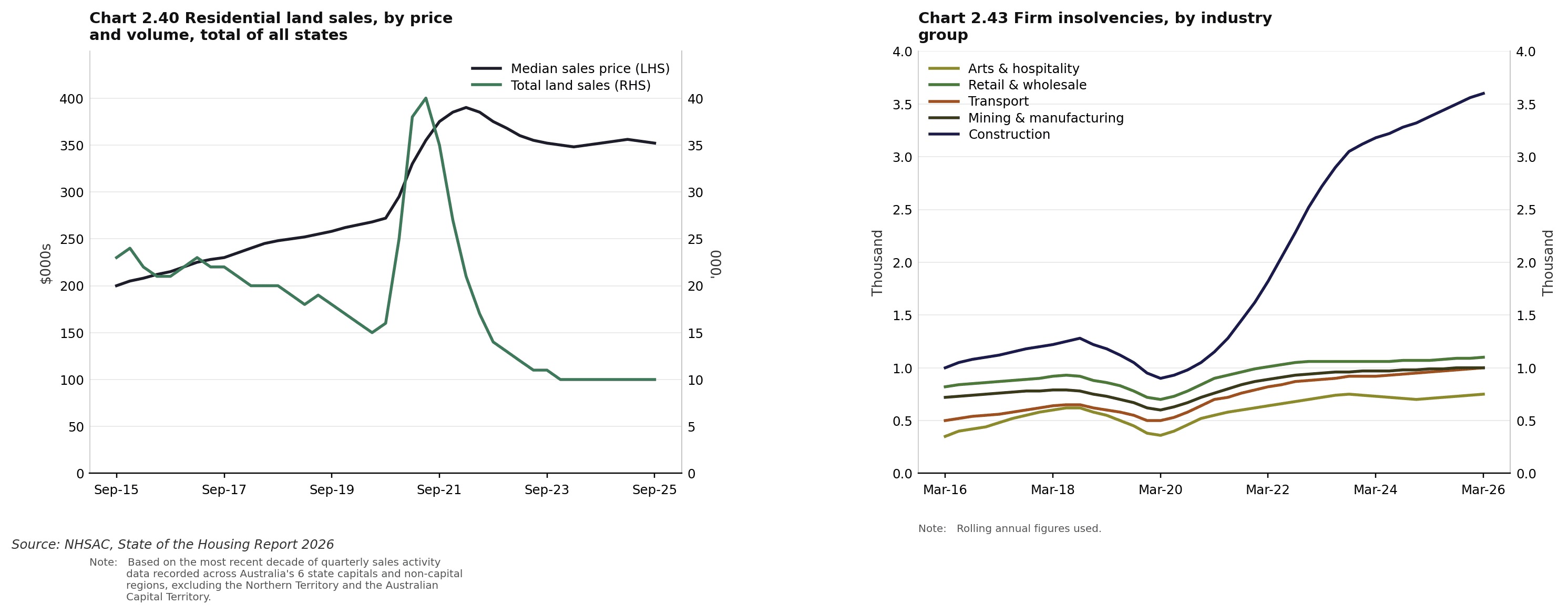
National data show residential land sales near decade lows, while median land prices have soared since 2020. Construction costs remain elevated, developers struggle to secure debt financing, and affordability constraints have reduced demand, contributing to longer wait times. These longer wait times add to project costs, as material and labour costs, as well as interest rates, can shift between signing and settlement. This matters because builders need demand to clear inventory and justify new projects. Together, these pressures have also contributed to higher insolvencies in the construction industry. 

The budget creates a wave of new demand for new builds. 

Buyers drawn into new-build markets are likely to be disproportionately investors (not owner-occupiers), whose primary motivation is to seek after-tax benefits. 

Builders could respond by raising prices and tailoring the product for investor buyers. 

When demand spikes amid constrained supply, builders gain pricing power, offering a solution for builders facing construction constraints. Consumers willing to pay a higher price view the tax deduction as sufficient justification for the higher cost. 

This raises a fair question: Are builders simply responding to genuine cost pressures, or are they capturing the benefits of current market conditions? 

The evidence from the most recent comparable policy experiment provides a reasonably clear answer. The 2025 HIA report found that government taxes, regulatory costs, and charges now account for up to 50% of the cost of a new house-and-land package in Sydney, 43% in Melbourne, and 41% in Brisbane. As discussed earlier, land costs have risen 3 times faster than inflation and 5 times faster than building material costs over the same period. 

On the surface, this supports the government’s stated rationale for the 2026 Budget: to preserve tax incentives for new supply and to direct investor demand towards dwellings that add to the housing stock rather than towards competing for existing homes. 

However, the most recent experiment, the “HomeBuilder” scheme, suggests this mechanism does not deliver the intended benefit. The RBA’s November 2021 statement concluded that new dwelling prices rose, driven by a substantial increase in builders’ material costs (excluding government subsidies) across most capital cities. Sustained demand from HomeBuilder enabled builders to pass cost increases through to buyers rather than absorb them. The ABS analysis of Producer Price Indexes between 2019 and 2024 found a consistent pattern, attributing the lift in house prices to the demand surge triggered by HomeBuilder and to historically low interest rates during COVID-19. 

This pattern isn’t unique to the HomeBuilder scheme. The 2022 AHURI report from the UNSW City Future Research Centre reviewed 25 years of Australian demand-side housing policy and concluded that, in a supply-constrained market, such measures consistently increase demand, driving up prices.

The 2026 Budget’s new build tax incentives are a demand-side measure applied to the same supply-constrained market. When demand is concentrated by a subsidy or tax incentive, and supply cannot respond at the same pace, the evidence suggests producers tend to capture a meaningful share of the benefit through higher prices. 

Builders face rising costs across the three major inputs: land, labour, and materials. While land and labour costs are largely shaped by market rates, materials, inclusions, and design choices offer more flexibility. In a tax-led purchase decision, the buyer may place greater weight on after-tax cash flow than on owner-occupier features such as generous storage, higher-spec finishes, or more considered layouts. This can make lower-cost specifications more commercially viable without necessarily reducing the headline price. The risk is that investors may pay a premium for a product whose value is supported more by tax treatment and rental yield than by the underlying build quality or long-term livability. 

The HIA argues for a supply-side alternative: reducing the tax burden on new home construction rather than stimulating demand for new homes. This would directly lower delivery costs and support affordability for both buyers and builders.

Investor saturation will build in these new-build pockets. 

The tax reforms specifically reward new builds, and buyers in these areas are disproportionately investors. Owner-occupiers do not receive the same tax benefit and have less incentive to pursue new builds in these locations. Over time, the suburb’s ownership composition could become heavily concentrated among investors. 

The resale problem arises when the first wave of investors tries to sell. 

The resale problem arises when the first wave of investors tries to sell. Two forces work against the seller. 

First, the new buyer cannot claim the same tax incentive because the property is no longer a new build under the policy definition. The tax treatment that justified the inflated purchase price no longer applies to the resale buyer, so the buyer cannot justify paying the same premium. 

Second, owner-occupiers are unlikely to step in and absorb the resale stock. Owner-occupiers typically lead the formation of suburbs, with investors following. In these new-build pockets, the order has been reversed. 

Picture an area built, designed, and lived in by owner-occupiers. Local schools, parks, shops, and services are shaped around permanent residents. Tenure is long, turnover is low, and the suburb’s human element becomes its pillar of stability.

Now, picture the inverse. An area built quickly, designed to a standardised template with limited variation between houses, and sold to investors who never set foot in the property. Where they exist, local facilities are sized for projected investor yields rather than community needs. Renters cycle through every 12-24 months. For-lease signs are a permanent feature of the streetscape. 

This is the human side of property that data alone can’t capture. This matters because just under 70% of Australian households are owner-occupiers. In a country where two-thirds of the buyer pool want to live in the property rather than collect rent, building stock designed for investors and rejected by owner-occupiers creates a self-limiting market.

This means the only buyers left at resale are other investors, who aren’t incentivised by the same tax benefits.

The outcome is weaker capital growth, rising vacancies and longer selling times. 

Investor-owned properties are part of the rental stock. As investors absorb new builds, more dwellings compete for tenants, but the tenant pool does not expand at the same pace. Vacancies rise, and rent growth is capped. On resale, if future buyers cannot match the premiums paid by the first wave, prices may grow slowly or stagnate, while days on market lengthen as sellers hold out for prices the next buyer cannot justify.

 Why does the chain hold together? 

Each link depends on the one before it. If builders were not supply-constrained, the demand wave would clear without price inflation. If demand were mixed, the suburb's composition would not shift. If post-2027 buyers could access the same tax treatment, resale premiums would persist. None of these conditions appears likely to hold post-budget, which is why the chain could translate into a measurable impact on investor returns.

The tax benefits captured during the holding period are real, but they apply to a smaller underlying gain. The next section tests this using a 10-year model that compares new-build and established properties under this theory.

Section 2: Modelling: New Build vs Established 10-Year Outcome

2.1. Model Assumptions

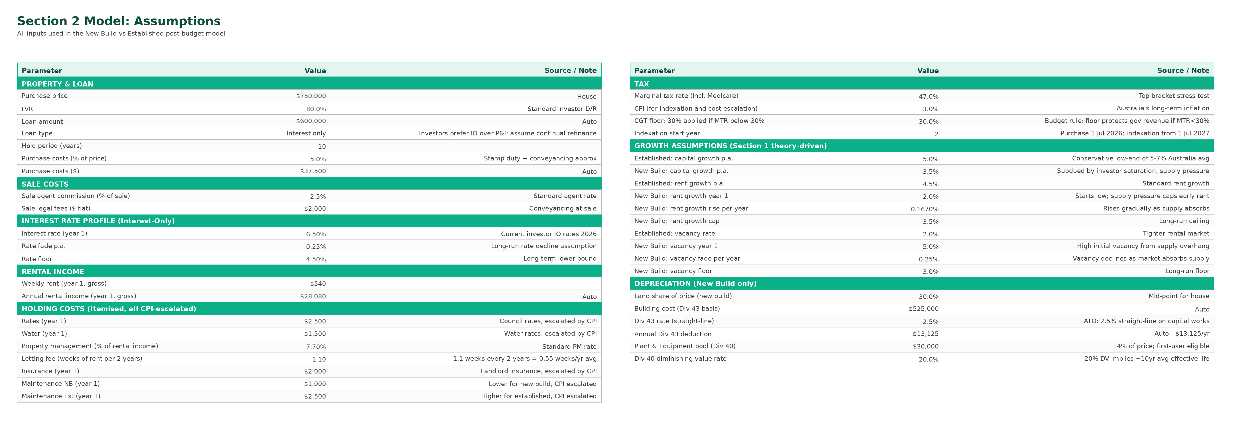
We have modelled two $750k properties purchased on 1 July 2026: one new build and one established house. Both are held for 10 years, sold in year 10, and financed with an 80% LVR interest-only loan. Both are owned by an investor in the 47% marginal tax bracket.

The market assumptions reflect the theory outlined in Section 1. New-build markets assume 3.5% p.a. capital growth and 5% vacancy (fading to 3% as supply is absorbed). Established markets grow at 5% p.a. (the conservative lower end of Australia’s long-term average of 5%-7%), with 2% vacancy, reflecting a balanced rental market. These assumptions are also stress-tested in Section 3 against historical market data, and the directional pattern appears to hold. 

Note: InvestorKit isn’t forecasting that every new-build market will underperform every established market by these exact margins. The model quantifies what could unfold if the chain of events described in section 1 plays out as expected. Individual markets may diverge from these assumptions in either direction. 

The full set of assumptions is shown below, with a brief note for each input.

2.2. Depreciation & Amortisation Schedule

These two schedules drive most of the year-on-year tax mechanisms: interest-only loan amortisation and the new build’s depreciation entitlement. 

For the established property, we have assumed no depreciation. This is a conservative assumption. In practice, established properties can still attract some depreciation benefits, particularly when investors make deductible repairs, touch-ups, or strategic renovations. 

For the new-build property, the investor claims capital works deductions under Division 43, calculated using the prime cost method, and plant and equipment deductions under Division 40, calculated using the diminishing value method, in line with ATO guidance.

The total depreciation over the 10-year holding period is $158k. This figure serves two purposes in the model: 

1. It reduces the new build’s taxable income each year, generating tax savings that improve after-tax cash flow

2. It reduces the new build’s cost base for CGT purposes at sale, which becomes relevant in section 2.5

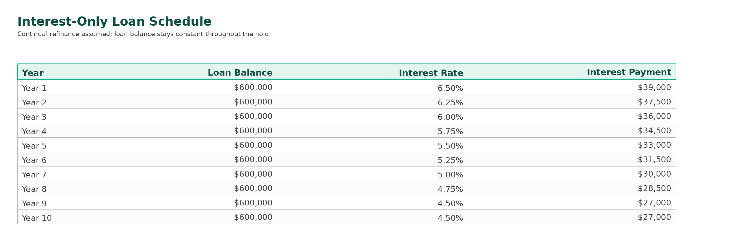
The model assumes the investor remains on an interest-only loan throughout the 10-year hold, so the $600k loan balance remains unchanged. Annual interest payments decline from $39k in Year 1 to $27k in Year 10, reflecting the modelled decline in interest rates from 6.5% to 4.5%. Both properties incur the same interest cost.

2.3. After-tax cash flow across the hold

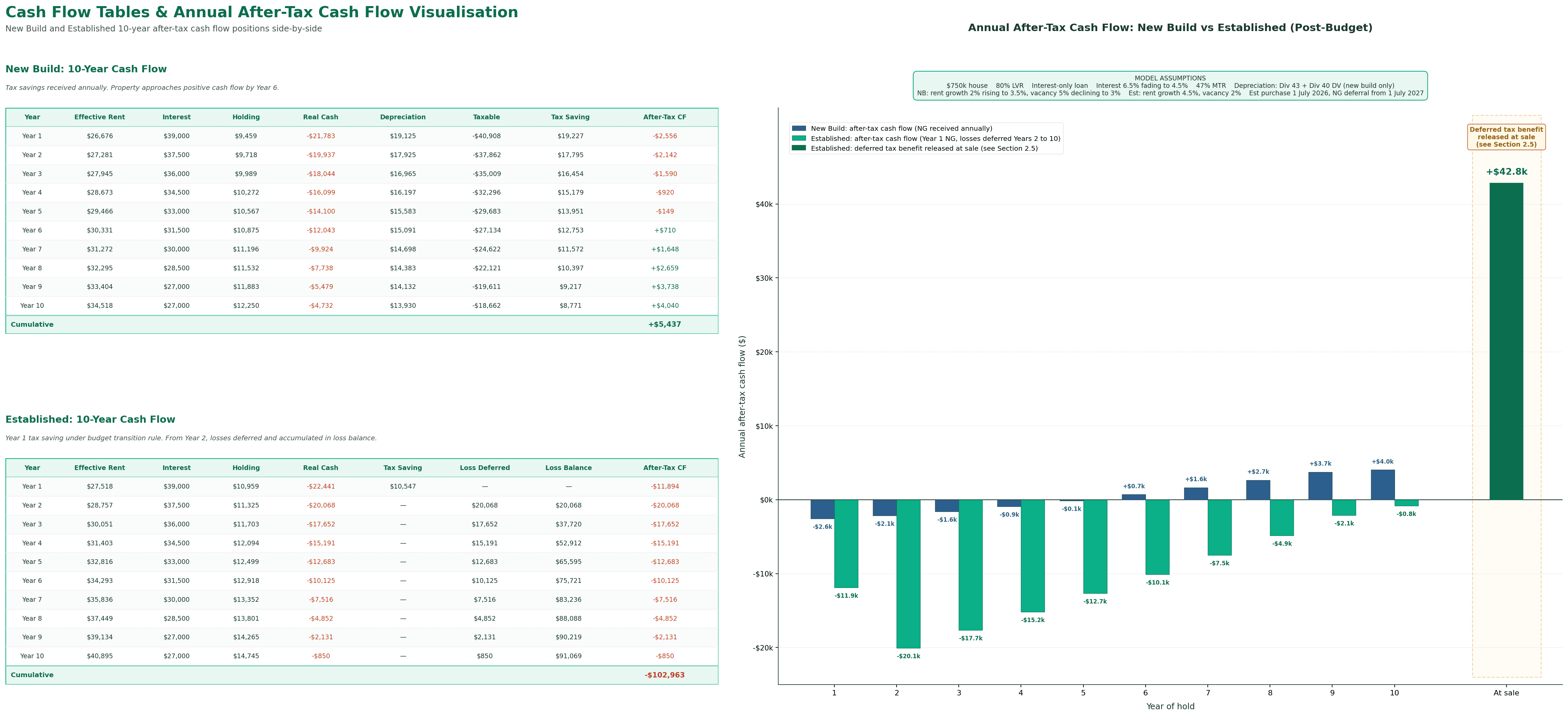
The new build is more comfortable to hold over the ownership period. It delivers negative gearing tax savings annually, starting at $19.2k in Year 1 and tapering to $8.8k by Year 10 as interest costs fall and rents rise. The depreciation component reduces the investor’s out-of-pocket holding costs and enables the property to reach positive after-tax cash flow by Year 6. By the end of Year 10, the new build has accumulated a marginal positive after-tax cash flow of roughly $5k.

The established property behaves differently. Year 1 still allows negative gearing under the budget’s transition rules, yielding $10.5k in tax savings. However, from Year 2 onwards, annual losses are deferred rather than offset against other income. As a result, the investor does not receive the same year-on-year tax relief during the holding period. Instead, the cash shortfall is recorded as a loss balance that grows each year and can be drawn down either when the property becomes cash-flow positive or at disposal. By Year 10, the property has accumulated a $91k loss balance, equivalent to a $42.8k tax offset if released at the investor’s 47% marginal tax rate.

Based on cash flow alone, the new-build property appears easier to hold. It requires less cash-flow support and reaches cash-flow positivity sooner. However, cash flow is only one part of the investment outcome. The capital growth and CGT components, covered next, determine whether this holding-period advantage translates into a stronger overall result over the long term.

2.4. Capital growth across the hold

At a $750k purchase price, the 1.5% growth differential (5% versus 3.5%) compounds to a $164k gap in property values by Year 10. The gap is barely visible early in the hold (just $11k in Year 1), reaches $66k by Year 5, and widens to $164k by Year 10. Compounding does the work here, not a single market event, which is why even a modest annual growth difference can translate into a material dollar outcome over a typical 10-year hold.

This is the single largest driver of the after-tax outcome. A reasonable question is whether a 1.5% growth gap is defensible. Section 3 addresses this by comparing Frankston (an established market) and Melton Bacchus Marsh (a new-build corridor) using Melbourne SA3 data. Over the past 10 years, the two markets recorded a 1.44% gap in median sales price growth and a 1.35% gap in median rent growth. Our 1.5% model assumption sits within this band rather than above it. 

2.5. CGT at sale

The capital growth trajectory directly feeds into the CGT calculation at the time of sale. Nominal capital gains are almost identical for the two properties, at $402k for the established and $373k for the new build. Despite this, the CGT bills diverge sharply. 

Two mechanisms drive the divergence in CGT payable. 

First, the new build's accumulated depreciation reduces its cost base. Total depreciation claimed over the hold is $158k, but only the Division 43 capital works portion ($131k) reduces the cost base under ATO rules. Subtracting the $131k Division 43 amount from the original cost base of $787,500 leaves an adjusted cost base of $656,250. This inflates the taxable gain on sale. This is why depreciation is not free money but a timing benefit. It improves annual cash flow during the hold, and part of that benefit is reconciled upon sale. The new build then elects the more favourable of the two CGT methods available to it: the 50% discount produces a $87.7k CGT bill, while indexation produces a $81.4k bill. The indexation method wins, and the investor pays $81.4k in CGT.

Second, the established property's $91k of accumulated deferred losses is released on sale and offsets the assessable gain before CGT applies. The real indexed gain of $162k is reduced to an assessable gain of $71k. This is not a new tax mechanism. The deferred loss carry-forward principle has been applied to trusts holding investment property for decades, with net capital losses carried forward and offset against future capital gains rather than written off. The 2026 Budget applies the same logic to individual investors who hold established residential property after 2027. 

Beyond the two mechanisms above, cost-based indexation also plays a meaningful role in reducing the CGT bill for both property types in this model. By applying a CPI uplift to the original purchase price over the holding period, indexation ensures the taxable gain reflects real growth rather than nominal growth. In this model, an indexation factor of 1.3048 (9 years of CPI at 3%) lifts the established property's cost base from $787,500 to $1,027,509, reducing a nominal gain of $402k to a real indexed gain of $162k before the deferred loss is applied. 

The new build also elects indexation over the 50% discount in this model, resulting in an $81.4k bill versus $87.7k from the 50% discount. Indexation does not eliminate CGT, but it ensures investors are not taxed on inflation. This mirrors how CGT operated in Australia before the 1999 introduction of the 50% discount, and how it continues to operate for trusts where the trustee is taxed at the top marginal rate.

The result is a $33k CGT bill for the established and an $81k CGT bill for the new build, a $48k CGT advantage in favour of the established at sale. This is the inverse of what most readers would expect after reading section 2.3. At the point of sale, the budget's transition mechanism reverses that pattern. The established deferred losses become a CGT shield, depreciation reduces the new build's cost base, and indexation strips inflation from the established gain. Three separate effects, all working against the new build at the point of sale.

2.6. Summary: Established property delivers nearly $100k more

The summary reconciles all covered components into a single after-tax outcome for each property.

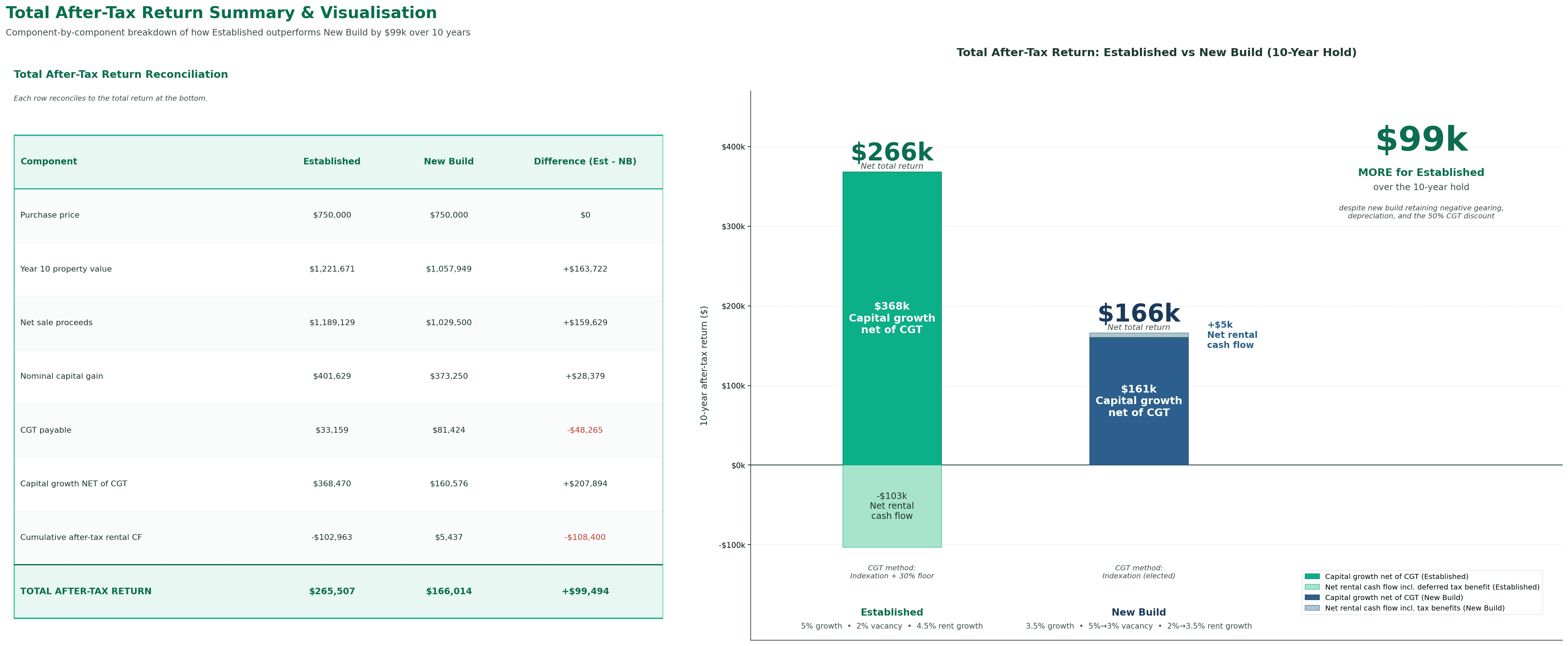
The established property delivers a net total return of $266k over the 10-year hold. The new build delivers $166k. The difference is nearly $100k in favour of the established, despite the new build retaining negative gearing, depreciation, and the 50% CGT discount. The new build wins on cash flow during the hold by $108k but loses on capital growth, net of CGT, by $208k. The capital growth advantage is roughly double the cash flow disadvantage, which is why the established finishes almost $100k ahead.

2.7 Stress Testing the Model

The table breaks down the 10-year after-tax return to identify the main driver of the superior returns of established property. For this stress test, the following are held constant: loan type, holding costs, purchase and aisles cost, and depreciation. 

• Equal Rent and Vacancy: Equalising rent growth and vacancy across both properties narrows the gap to $81,704, confirming that rental cash flow is a contributor, but not the primary driver. 

• Equal Capital Growth: The new build is given the same capital growth rate as the established property; the outcome is reversed, and the new build finishes $16,381 ahead. 

This indicates that the established property's advantage in this model is driven by the capital growth differential rather than by tax treatment. 

Section 3: Three Historical Case Studies

Section 2 models what could unfold after the budget if the chain of events described in Section 1 plays out as expected. The model rests on three central assumptions: 

• New-build capital growth 1.5% below established

• Elevated vacancy rates in new-build markets (fading as supply is absorbed)

• Slower rent growth in saturated new-build markets

This section grounds each assumption in historical evidence. The three selected case studies demonstrate the same dynamic across Australia at the market level (SA3), property level (matched pair), and long-term trajectory (suburb maturation). 

The point is not that every new-build market will underperform by these exact margins, but that the pattern the model assumes is not theoretical. It has happened before, in conditions that mirror those the 2026 budget is now setting up, and the historical outcomes are at or beyond the model's assumptions for the post-budget environment. 

3.1. Frankston vs Melton Bacchus Marsh: the same dynamic, 10 years earlier

This case study compares two Melbourne SA3 markets over the same 10-year period (Jan 2015 to Jan 2025). Frankston is a mature, established residential market in Melbourne’s south. Melton Bacchus Marsh is a new-build corridor that’s heavily oversupplied and located in Melbourne’s far west. Both markets are within Greater Melbourne. 

Frankston recorded 6.88% annualised growth over the past decade, compared with 5.44% in Melton Bacchus Marsh (a 1.4% gap). For rent growth, Frankston grew at 5.44% p.a and Melton Bacchus Marsh at 4.14% (a 1.35% gap). Our model assumed a 1.5% growth differential between established and new-build markets, and the Frankston vs Melton data sits just below that at both price and rent levels.  

The third and fourth panels explain the oversupply risk associated with new builds. Frankston’s BA rate averaged 0.49%, while Melton Bacchus Marsh averaged 9.26%, peaking at 14.95%, over the decade. 

Building approvals on their own aren’t the problem. The risk arises when approvals outpace demand absorption, and the inventory panel confirms this for Melton Bacchus Marsh. Inventory peaked at 13 months in early 2019 and did not return to the balanced range until 2021. Frankston, by contrast, remained at or below the balanced range for the full decade. 

This is the structural condition Section 1’s theory identifies. When supply runs that far ahead of demand for that long, vacancy remains elevated, rent growth lags, and capital growth compounds more slowly. 

These markets produced this dynamic because the conditions at the time were similar to those the 2026 Budget could now create. 

First, investor lending reached its highest concentration on record. ABS data show that the investor share of new housing loan commitments peaked at 45.9% in 2015, just before APRA’s macroprudential intervention, which imposed a 10% speed limit on investor credit growth. At that peak, nearly half of newly originated housing loans were for investors, the highest concentration ever recorded. 

Second, the Treasury Laws Amendment Bill (Housing Tax Integrity) Bill 2017 removed Division 40 deductions for previously used plant and equipment when purchasing any second-hand residential property. Before this change, an investor’s tax position did not strongly favour new builds over established properties. The investor tilt towards new builds during this period stemmed from yield, affordability and developer incentives. 

Third, building approvals in Melton, Bacchus Marsh and the surrounding corridor were running at multiples of established market levels. Supply outpaced demand, and it took time for demand to absorb the excess supply. 

These conditions aren’t 100% identical to the post-2026 Budget environment, but the structural dynamics are the same. A concentrated wave of investor demand meets a supply-constrained new-build environment, leading to weaker capital and rental growth at the corridor level than in established markets within the same metropolitan area. 

The 1.4% price gap currently sits just below the model’s 1.5% assumption. If anything, the model’s assumption is conservative compared with what a comparable Melbourne SA3 could deliver over the same 10-year window. 

3.2. Tarneit matched pair: the same dynamic, within a single suburb

One could argue that two SA3s differ in factors beyond build composition, such as distance to the CBD, access to employment, demographics, and amenities. To address this objection, the second case study compares 2 houses in the same suburb. 

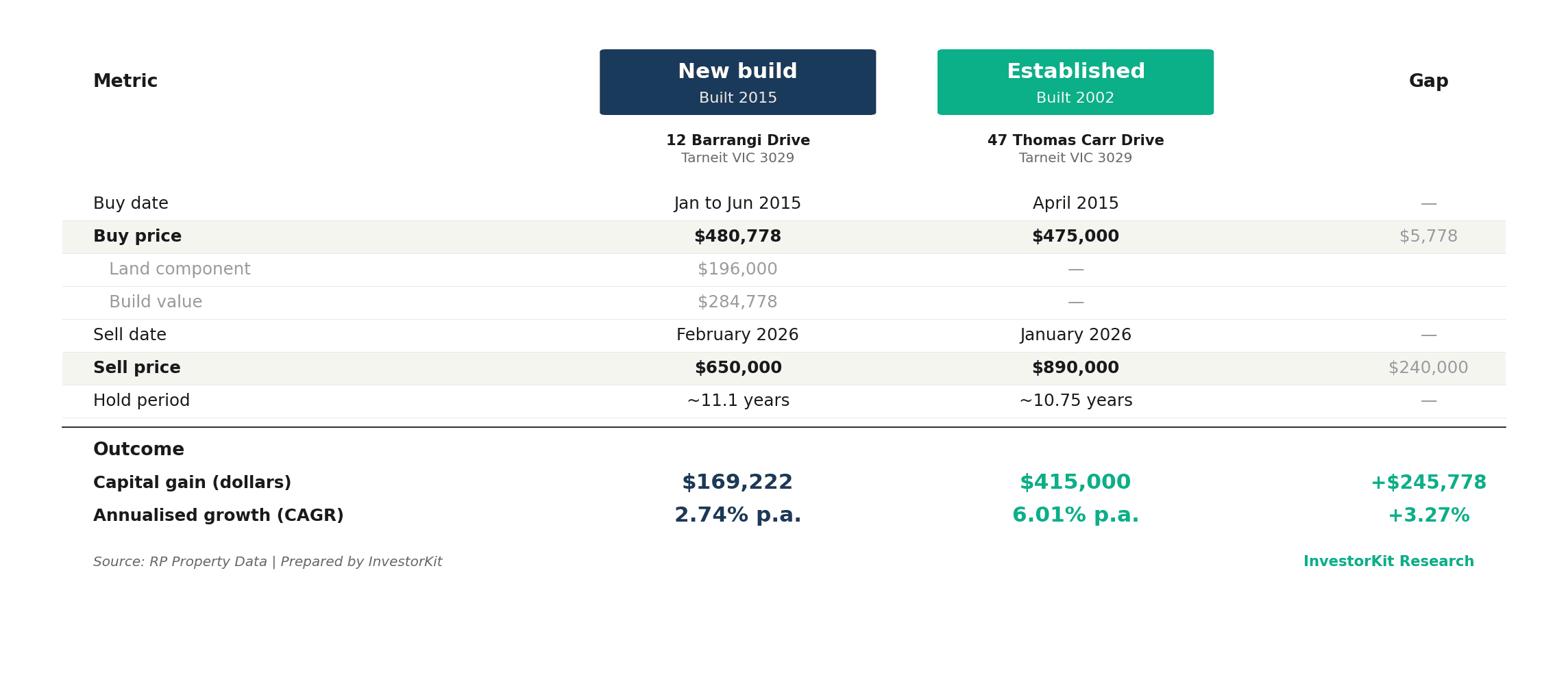
Two houses in Tarnet, VIC 3029, were purchased in the first half of 2015 at nearly identical prices. Both are 4-bedroom, 2-bathroom, 2-car houses. When sold again 11 years later, the new build sold in February 2026 for $650k, and the established house sold in January 2026 for $890k (with no renovation). 

Same suburb, same dwelling structure, similar holding period, and starting price. The only meaningful variance is the year built. The established delivered $415k in capital gains, compared with $169,222 for the new builds, a $245,778 difference. Annualised, the new build grew at only 2.74%, while the established grew at 6.01% (a 3.27% gap). 

This is a single matched pair, not a statistical sample, so it is a cherry-picked example. The point is not that every new vs established property in Tarnet shows a 3.27% gap, but that such a gap can exist at the property level, even within the same suburb, when build age is the only variable.

In addition, new builds typically have a lower land-to-asset ratio than established stock. Since land appreciates over time while buildings depreciate, a property with a lower land share has a smaller proportion of its value in the component that drives capital growth. Instead, more of the value is reflected in the price premium, which includes developer margins, sales commissions and tax-incentive pricing. 

3.3. North Lakes new build market maturatisation story

The first two case studies demonstrate the same dynamic over a 10-year hold period. A reasonable counter-argument is that new-build markets eventually mature and no longer behave as new-build markets. The third case study illustrates what maturation looks like in practice and how long it may take. 

North Lakes, QLD, is a master-planned community. The masterplan was launched in 1999, and the completion phase was finalised in 2017. The case study tracks 4 metrics across the suburb’s life cycle: median sales price, weekly rent, building approval rate and rental vacancy rate.

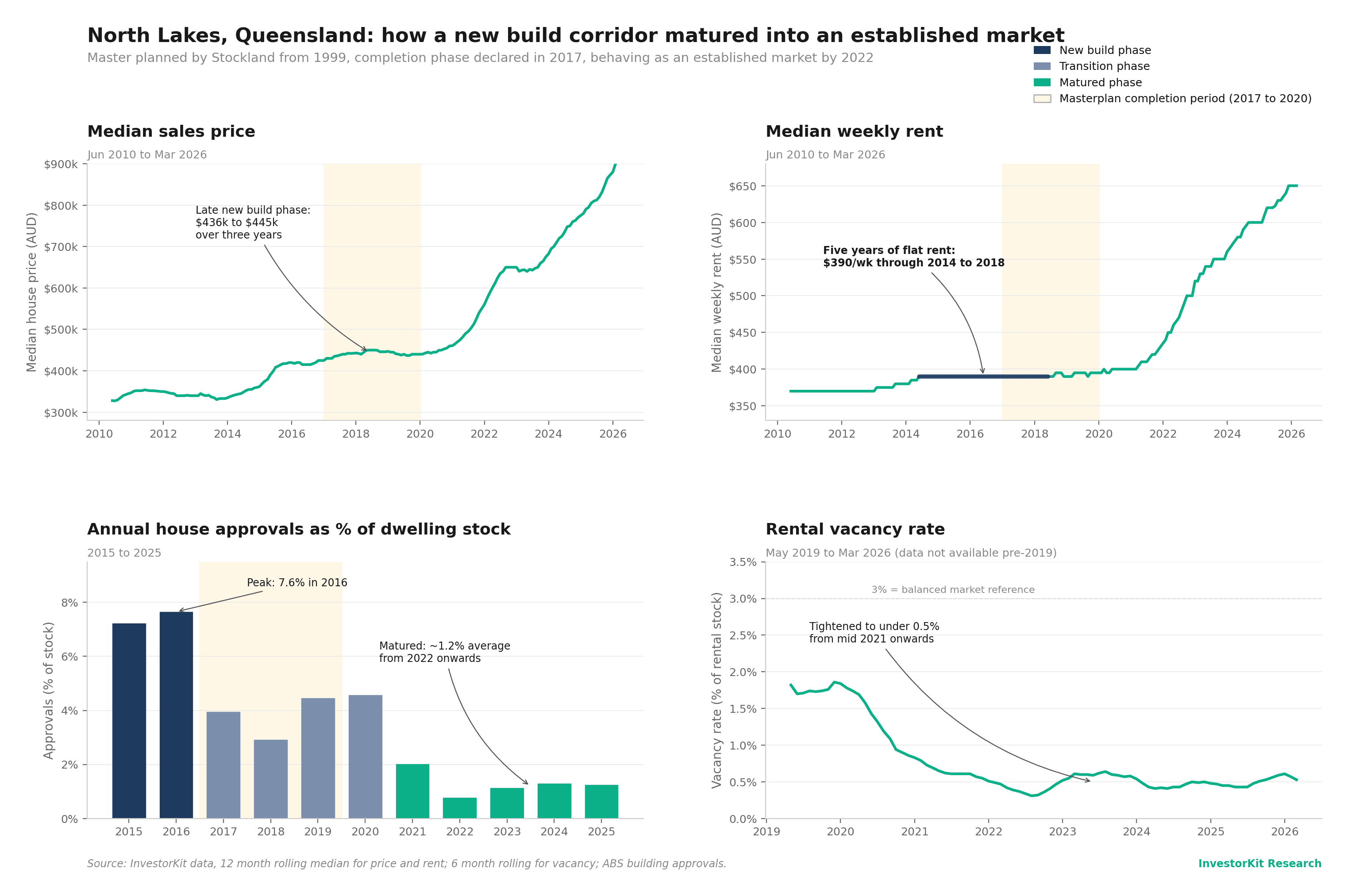
 Median house prices rose from $322k to $445k between 2010 and 2016, then plateaued for 3 years during the masterplan completion period, when a large stock entered the market. Only from 2021 onwards, years after the masterplan was completed and the market had absorbed the supply, did prices start accelerating, reaching close to $900k by early 2026. 

The rent chart shows the same pattern. Median weekly rent remained unchanged at $390 from 2014 to 2018. Rents began to move in 2020, accelerating in 2022 after the suburb had matured. 

The building approvals and vacancy charts explain this mechanism. North Lakes was a master-planned community by design, so supply was expected to spike during the build-out phase. Building approvals peaked at 7.6% in 2016, the peak of the late new-build phase, before falling to roughly 1.2% in the mature phase from 2022 onwards. 

The demand couldn’t absorb the supply at the rate it arrived. Vacancy rates remained between 1.5% and 2% from 2019 to 2020. Medinan rents remained flat at $390 for 5 years, from 2014 to 2018, and sales prices plateaued for 3 years during the masterplan completion period (2017 to 2020). 

Building approvals on their own didn’t produce these outcomes. A masterplan corridor that was supply-heavy by design led to incoming supply outpacing demand absorption. 

The takeaway isn’t that North Lakes is a bad market. It eventually became a strong, established market. Its recent 5-year annualised growth of 14.3% indicates strong price acceleration. The takeaway is the timing. A property purchased during the new-build phase (2014 to 2020) sat for several years with low capital and rental growth before the maturation phase delivered returns. That same capital, deployed in an established market with healthy market pressure and a strong local economy, would have started compounding from year 1.  

Section 4: Conclusion

The 2026 Federal Budget changed the tax rules, not the property fundamentals. Investors don’t invest for tax deductions. They invest for capital growth, equity build-up, and potential early retirement.

Capital growth determines the size of the underlying gain that is taxed first. As noted earlier, a larger gross gain, taxed less favourably, can still deliver more dollars than a smaller gross gain taxed more favourably. The model in section 2 demonstrated this, and the historical case studies in section 3 support it. 

If you can manage cash flow, the established property pulls ahead in the long run as rents rise and interest rates normalise in the coming years. Both factors reduce holding strain over time. In addition, the deferred losses do not disappear; they are released at sale to offset the capital gain, and indexation strips inflation from the cost base before the gain is calculated. 

This is the fundamental reason InvestorKit’s strategy does not pivot when the government changes tax rules. Our buying decisions are anchored in market fundamentals, not tax incentives. When tax policy shifts, the fundamentals that drive capital growth do not shift with it.

When the data show that new builds are structurally engineered to deliver sustainable, long-term returns that compete with those of established properties, we will revise our strategy. That day has not arrived. 

If you want to discuss what a research-led, established property strategy looks like for your portfolio, our buyer’s agency team offers a free 15-minute discovery call.